

【Excerpt Note】Population Encoding and Decoding
The content is from the lecture notes (M1_Slides_Population_Coding, M1_Notes_Population_Coding) of ‘Theoretical Systems Neuroscience’ by Professor Wei Ji Ma (Baylor College of Medicine) in 2013. He is now leading the Wei Ji Ma’ lab at Center for Neural Science and Department of Psychology at New York University.
For further more info on the course website CAAM/NEUR 415: Theoretical Neuroscience Fall 2013, Biophysical Modelling and Computation from Cell to Network at Rice University.
Some useful MATLAB example of population coding and decoding from the Book, Gabbiani, Cox: Mathematics for Neuroscientists , 1st Edition.
Table of Contents
1 Population encoding and decoding
1.1 Encoding
1.2 Decoding
1.2.1 Winner‐take‐all decoder
1.2.2 Center‐of‐mass or population vector decoder
1.2.3 Template‐matching decoder
1.2.4 Maximum‐likelihood decoder
1.2.5 Bayesian decoders
1.2.6 Sampling from the posterior
1.3 How good are different decoders?
1.3.1 Cramér‐Rao bound
1.3.2 Fisher information
1.3.3 Goodness of decoders
1.3.4 Neural implementation
1.4 Decoding probability distributions
1.4.1 Other forms of probabilistic coding
1.4.2 Discrete variables
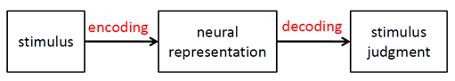
A population code is a way of representing information about a stimulus through the simultaneous activity of a large set of neurons sensitive to the feature. This set is called a population. A population code is useful for increasing the animal’s certainty about a feature, as well as for encoding multiple features at once. Encoding is how a stimulus gives rise to patterns of activity (in a stochastic manner), decoding is the reverse process, by which a neural population is “read out”, either by an experimenter or by downstream neurons, to produce an estimate of the stimulus. Population codes are believed to be widespread in the nervous system.
1. Population Encoding and Decoding
-
Stimulus: physical feature of the world (often 1D)
- Orientation of a contour
- Direction of self-motion
- Number of students in class
- Whether object A is bigger than object B
- ……
- Neural Representation: spike activity of neurons in response to stimulus (population code)
- Stimulus judgment: often motor response
1.1 Encoding
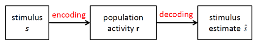
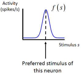
Let s be the stimulus (or a specific value of the stimulus). We will denote the response of a neuron to the stimulus by r. For a brief stimulus, this is the total number of spikes elicited. For a sustained stimulus, it can be the total number of spikes in a certain time interval. When s is presented many times, different values of r will be recorded. We will denote the mean response by f(s). Unlike r, f(s) is not necessarily an integer. As a function of s, f(s) is called the tuning curve of the neuron. It typically is bell‐shaped (for stimuli like orientation) or monotonic. When it is bell‐shaped, then the mode of the function is called the preferred stimulus of the neuron. The variability of r around its mean in response to s can often reasonably be described as a Poisson process with mean f(s). That means that it is drawn from the following distribution:
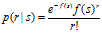
Note that this is a conditional probability distribution: we are not interested in the distribution of responses in general, but only in response to a specific stimulus. The variance of a Poisson-distributed variable is equal to its mean, which is not completely consistent with measurements. In most cortical neurons, the Fano factor, which is the ratio between variance and mean, is found to be more or less constant over a range of mean activities, but with a value anywhere between 0.3 and 1.8.
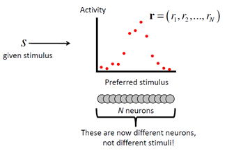
Different neurons will in general have different tuning curves. Suppose we have a population of n neurons. We label the neurons with an index i, which runs from 1 to n. The tuning curve of the i’th neuron is denoted fi(s). Instead of choosing a Poisson distribution to describe neural variability, one can use a normal distribution:
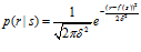
For large values of the mean, a Poisson distribution is very similar to a normal distribution. A normal distribution can be made into a more realistic description of variability by taking its variance to be proportional or equal to its mean, just as is the case for the Poisson distribution. However, for small values of the mean, any normal distribution runs into problems since it is defined on the entire real line, including negative values, whereas spike counts are always nonnegative. One can cut it off at zero, but then the distribution loses the nice properties of the normal distribution.
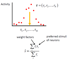
On a single trial, the response of a single neuron is denoted ri, and the population response can be written as a vector r = (r1,…,rN). We can characterize the variability of the population response upon repeated presentations of stimulus s by a distribution p(r|s). This is called the response distribution or the response distribution, although the word “noise” might be misleading. In more generality, a mathematical description of how the observations are generated probabilistically by a source variable is called a generative model.
The simplest assumption we can make to proceed is that variability is independent between neurons. This means that for a given s, the probability distribution from which a spike count in one neuron is drawn is unrelated to the activity of other neurons. In that case, the response distribution of the population is a product distribution:

Tuning curve of a single neuron
Mean response as a function of the stimulus
Population activity on a single trial
1.2 Decoding
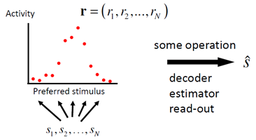
Based on a pattern of activity r, the brain often has to reconstruct what was the stimulus s that gave rise to r. This is called decoding, estimating, or reading out s. There are many ways of doing this, some of which are better than others.
Decoding population activity
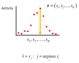
1.2.1. Winner-take-all decoder
Suppose that each neuron in the population has a preferred stimulus value. Then, a simple estimator of the stimulus is the preferred stimulus value of the neuron with the highest response:
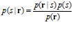
1.2.2. Center-of-mass decoder
A better decoder is obtained by computing a weighted average of the preferred stimulus values of all neurons, with weights proportional to the responses of the respective neurons: each neuron “votes” for its preferred stimulus value with a strength proportional to its response:
While this method performs quite well in many cases, it does not take the form of neuronal variability into account. On a circular stimulus space – for instance when the stimulus is orientation or motion direction – the equivalent of this method is called the population vector. It has been applied to experimental data, for instance by Georgopoulos et al. (Georgopoulos,Kalaska et al. 1982) to decode movement direction from population activity in primate motor cortex.
1.2.3. Template-matching decoder
We can ask the question for which stimulus value s the observed population response is closest to the mean population response generated by s. That is, we match the observed population response with a set of templates (mean population responses for different s). As an error measure, we use the sum‐squared difference. This gives the decoder


This decoder also does not take the form of neuronal variability into account, but uses more than only the preferred stimulus values of the neurons.
1.2.4. Maximum-likelihood decoder
An important method that does take the form of neuronal variability into account is the maximum‐likelihood decoder. This decoder computes the probability that a stimulus value elicited the given population response, and selects the stimulus value for which this probability is highest:

1.2.5. Bayesian decoders
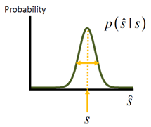
Bayesian decoders use Bayes’ rule to express the probability of a stimulus given a response, p(s|r), as the normalized product of the probability of this response given a stimulus, p(r|s), and the prior probability of the stimulus, p(s):
The prior probability reflects knowledge about the stimulus before the population response is elicited, and can have been generated on the basis of previous experience. The probability distribution obtained in this way is referred to as the posterior probability distribution over the stimulus. When the number of neurons is large, this distribution is usually a narrow normal distribution. It can be collapsed onto an estimate by taking the value that has the highest posterior probability; this is called the maximum‐a‐posteriori (MAP) decoder (also the mode of the posterior):

1.3 How good are different decoders?
Given that there are so many possible decoders, how can we objectively evaluate how good each of them is? Imagine you have a large number of population patterns of activity all generated by the same value of s. For each pattern, you apply your decoder of interest to obtain an estimate sˆ . Now look at the distribution of estimates, p(sˆ | s). There are several criteria for what makes a decoder good. First, you would like the mean estimate to be equal to the true stimulus value, i.e. sˆ = s . Here, the average ⋅ is in principle over p (sˆ | s) but can also be regarded as one over p(r|s), since ˆs is a function of r for all deterministic decoders (but not for the sampling decoder). The difference between the mean estimate and the true stimulus value is called the bias of the estimator, and it may depend on s:

An estimator is called unbiased if b(s)=0 for all s. It is not very difficult for a decoder to be approximately unbiased. Most of the decoders we described in the previous section are unbiased in common situations. However, not all unbiased decoders are equally good, since not only the mean matters, but also the variance. The smaller the variance, the better the decoder. Whereas bias can be equal to zero, this is not true for the variance – because of variability in patterns of activity, it is impossible for an unbiased decoder to have zero variance. (It is easy for a biased decoder to have zero variance: just take one that ignores the data and always produces the same value. This decoder has no variability, but it is severely biased for all values of s but one.) It turns out that there is a fundamental lower bound on the variance of an unbiased decoder. This is a famous result in estimation theory, known as the Cramér‐Rao inequality. We will go through it in some detail because it is an important notion in population coding.
Good decoders
- Unbiased
- Low variance
- Can be implemented by a neural network.
1.3.1. CramérRao bound
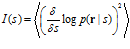
Based on the response distribution p(r|s), one can define a quantity called the Fisher information that the population contains about s:
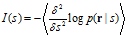
where ∂ denotes a partial derivative and the average ⋅ is now over p(r|s). Fisher information can alternatively be expressed as

This is the Cramér‐Rao bound (or inequality). It states that no estimator ˆs can achieve a variance that is smaller than the inverse of the Fisher information. An estimator that has the smallest possible variance is called an efficient estimator. The Cramér‐Rao bound can be generalized to multidimensional (vector) variables.
1.3.2. Fisher information
Since Fisher information puts a hard limit on the performance of any possible decoder, it is a decoder‐independent measure of the information content of a population of neurons (which is why it is called “information” in the first place). Here, the understanding is that the population is characterized by its response distribution. Fisher information reflects the maximum amount of information that can be extracted from a population. The variance of an estimator determines the smallest change in the stimulus that can be reliably discriminated. If the variance is small, the estimator can be used to detect tiny changes in s. Accordingly, there is a link between Fisher information and discrimination threshold: Fisher information is inversely proportional to the square of the discrimination threshold of an ideal observer of the neural activity, or equivalently, it is proportional to the square of the sensitivity d ‘ of an ideal observer:

where d ‘ is the sensitivity (a measure of performance) and δ s is the distance between the two stimuli to be discriminated. Fisher information is subject to the data processing inequality, which states that no operation on the data (in our case population patterns of activity) can increase Fisher information.
Note: the Fisher information (https://en.wikipedia.org/wiki/Fisher_information ) may be seen as the curvature of the support curve (the graph of the log-likelihood). Near the maximum likelihood estimate, low Fisher information therefore indicates that the maximum appears “blunt”, that is, the maximum is shallow and there are many nearby values with a similar log-likelihood. Conversely, high Fisher information indicates that the maximum is sharp.
1.3.3. Goodness of decoders
There are some general results that are helpful here. It turns out that in the limit of a large number of observations (in our case, many spikes), the maximum‐likelihood estimate is the “best possible” one in the sense that it is both unbiased and efficient. Moreover, its distribution is approximately normal in this limit.
Other decoders will have a larger bias and/or a larger variance than the maximum‐likelihood decoder, although in simple situations, some of them may come very close. Typically, the winner‐take‐all decoder and the sampling decoder are rather poor, but one might choose them for their computational advantages.
1.3.4. Neural implementation
So far, we have discussed many decoders from an abstract perspective. However, the brain itself also has to do decoding, for example in generating a response to a stimulus. Therefore, if we want to know whether a particular decoder is used in performing a perceptual task, the question needs to be answered how it can be implemented in neural networks. Fortunately, this problem has been solved for the maximum‐likelihood decoder. Under certain assumptions on the form of neural variability, a line attractor network can turn a noisy population pattern of activity into a smooth pattern that peaks at the maximum‐likelihood estimate (Deneve, Latham et al. 1999).
The winner‐take‐all decoder can easily be implemented using a nonlinearity (to enhance the maximum activity) and global inhibition (to suppress the activity of other neurons). Neural implementations of the other decoders we discussed are not known.
1.4 Decoding probability distributions
Further info in the lecture notes.
Deneve, S., P. Latham, et al. (1999). “Reading population codes: a neural implementation of ideal observers.” Nature Neuroscience 2(8): 740‐745.
Foldiak, P. (1993). The ‘ideal homunculus’: statistical inference from neural population responses. Computation and Neural Systems. F. Eeckman and J. Bower. Norwell, MA, Kluwer Academic Publishers: 55‐60.
Georgopoulos, A., J. Kalaska, et al. (1982). “On the relations between the direction of twodimensional arm movements and cell discharge in primate motor cortex.” Journal of Neuroscience 2(11): 1527‐1537.
Pouget, A., P. Dayan, et al. (2003). “Inference and Computation with Population Codes.” Annual Review of Neuroscience. Sanger, T. (1996). “Probability density estimation for the interpretation of neural population codes.” Journal of Neurophysiology 76(4): 2790‐3.
Zhang, K., I. Ginzburg, et al. (1998). “Interpreting neuronal population activity by reconstruction: unified framework with application to hippocampal place cells.” Journal of Neurophysiology 79(2): 1017‐44.