
How to update the activity of pose cells in RatSLAM?
The excerpt note is from Michael et al., 2008, which explains the detail process to update the activity of pose cells in RatSLAM.
Milford, Michael J., and Gordon F. Wyeth. “Mapping a suburb with a single camera using a biologically inspired SLAM system.” IEEE Transactions on Robotics 24, no. 5 (2008): 1038-1053.
The pose cells form the core of the RatSLAM system. The pose cells represent the three degree of freedom (DoF) pose of the robot using a three-dimensional version of the CAN. Each face of the three-dimensional pose cell structure is connected to the opposite face with wraparound connections.
Activity in the pose cells is updated by self-motion cues, and calibrated by local view. The self-motion cues are used to drive path integration in the pose cells, while the external cues trigger local view cells that are associated with pose cells through associative learning. In this study, both the local view and the self-motion cues are generated from camera images.
The activity in the pose cells is described by the pose cell activity matrix  , and is updated by the attractor dynamics, path integration, and local view processes.
1) Attractor Dynamics
The process of attractor dynamics including Local Excitation, Local Inhibition, Global Inhibition, Global Normalization.
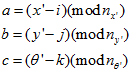
A three-dimensional Gaussian distribution is used to create the excitatory weight matrix , where the indexes a, b and c represent the distances between units in
  ,
, and
and  coordinates, respectively. The distribution is calculated by
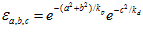 (1)
(1)
Where  and
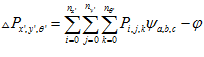
and  are the width constants for place and direction, respectively. The change of activity in a pose cell due to local excitation is given by (note: these indexes must be set to n-1 so that formula (3) will work)
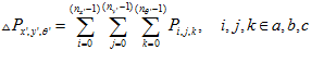 (2)
(2)
Where  are the three dimensions of the pose cell matrix in
  space. The calculation of the excitatory weight matrix indexes cause the excitatory connections to connect across opposite faces; thus
 (3)
(3)
The computation of (2) across all pose cells is potentially expensive, as it represents a circular convolution of two three-dimensional matrices. Significant speedups are achieved by exploiting the sparseness of the pose cell activity matrix; for the parameters used in this paper, typically around 1% of cells have nonzero values.
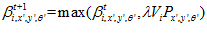
Each cell also inhibits nearby cells using an inhibitory form of the excitatory weight matrix, with the same parameter values, but negative weights. By performing inhibition after excitation (rather than concurrently), and adding slight global inhibition, the symmetry of the excitatory and inhibitory weights leads to suitable network dynamics, without using traditional Mexican hat connectivity. Consequently, the network is easier to work with, not requiring separate tuning of different excitatory and inhibitory weight profiles. The slight global inhibition is applied equally across all cells, with both inhibition processes given by
 (4)
(4)
Where  is the inhibitory weight matrix and
  controls the level of global inhibition. All values in
  are then limited to nonnegative values and normalized.
Without external input, the activity in the pose cell matrix converges over several iterations to a single ellipsoidal volume of activity, with all other units inactive.
The next two sections briefly describe how activity can shift under a process of path integration, and how activity can be introduced by local view calibration.
2) Path Integration
Rather than computing weighted connections to perform path integration, RatSLAM increases both the speed and accuracy of integrating odometric updates by making an appropriately displaced copy of the activity packet. This approach sacrifices biological fidelity, but computes faster, has no scaling problems, and does not require particularly high or regular update rates. Note that unlike probabilistic SLAM, there is no notion of increasing uncertainty in the path-integration process; the size of the packet does not change under path integration. Path integration for the studies is based on visual odometry signals.
3) Local View Calibration
The accumulated error in the path integration process is reset by learning associations between pose cell activity and local view cell activity, while simultaneously recalling prior associations. The local view is represented as a vector V, with each element of the vector representing the activity of a local view cell. A local view cell is active if the current view of the environment is sufficiently similar to the previously seen view of the environment associated with that cell.
The learnt connections between the local view vector and the three-dimensional pose cell matrix are stored in the connection matrix  . Learning follows a modified version of Hebb’s law where he connection between local view cell
  and pose cell
  is given by
 (5)
(5)
Which is applied across all local view cells and pose cells that are active. The change in pose cell activity under calibration is given by
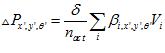 (6)
(6)
Where the  constant determines the strength of visual calibration, and
  is the number of active local view cells.
4) Local View Cell Calculation
A local view cell is active if the current view of the environment is sufficiently similar to the previously seen view of the environment associated with that cell. In the implementation described in this paper, the current view is compared to previous views using the same scanline intensity profile that formed the basis of odometry. Previously seen scanline intensity profiles are stored as view templates with each template paired to a local view cell. The current scanline intensity profile is compared to the stored templates, and if a match is found, the local view cell associated with the matching stored template is made active. If there is no match to a previously seem template, then a new template is stored and a new local view cell created that is associated with the new template.
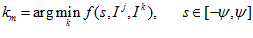
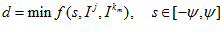
The comparison between the current profile and the templates is performed using the average absolute intensity difference function. The comparison is performed over a small range of pixel offsets  to provide some generalization in rotation to the matches. The best match is found as
 (16)
(16)
Where  is the current profile and
  are the stored profiles,
  is pixel offset. The quality of the match
  is calculated by
 (17)
(17)
And tested against a threshold  to determine whether the profile is sufficiently similar to the template or whether a new template need be created, and
  updated accordingly. The local view vector is then set
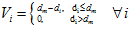 (18)
(18)
For further info, pleasure read the Michael and Gordon 2008.
Milford, Michael J., and Gordon F. Wyeth. “Mapping a suburb with a single camera using a biologically inspired SLAM system.” IEEE Transactions on Robotics 24, no. 5 (2008): 1038-1053.